Euclidean Shortest Path Problem

Abstract:

In the new corporate world, time is everything. An optimized way of working is vital. Similarly, in Computer Science an algorithm that is practical, easy and best solves the problem is necessarily not optimal if it runs in exponential time. Nevertheless, an algorithm that is more complex but solves the same problem in constant time is more valuable. Therefore, generating an optimal solution to any problem in any field is fundamental to our life. Finding the shortest path falls in the same line, being crucial to spatial analysis and wayfinding tasks. When you are driving from City A to City B using Google maps, Google maps automatically routes you to the path that takes the least time to reach the destination. This routing is based on the problem of finding the shortest path. This problem is also used to compute the shortest path on the road networks of the USA and Europe. In the field of networking, the shortest path algorithm is used to find the minimum delay. The other applications of this problem include Robotics, VLSI, and transportation.

Introduction:

Distance, being a description of how far objects lie from each other in terms of physical length, needs a definite and efficient measure to it. Since our data is in a numerical format, distance measures like Binary distance, Euclidean distance, Squared Euclidean distance, Manhattan distance, Minkowski distance (a generalized metric form of Euclidean distance and Manhattan distance), Cosine distance, Correlation distance, etc can be used. Amongst all of these Euclidean distance is the one most commonly used and that is the one we have made use of in this project as well. Euclidean distance gives the length of the segment or straight path connecting two points. In two dimensional space, the Euclidean distance between two points (a1, b1) and (a2, b2) is given by the Euclidean distance formula given below.

sqrt[(a2 - a1)^2 + (b2 - b1)^2]

Our project is based on the Euclidean shortest path problem in Computational Geometry. The problem space contains a set of polyhedral obstacles in Euclidian space and a starting point and an ending point. The Euclidean shortest path algorithm should find a path between the two points such that no point in path intersects any of the obstacles. This problem is also called a mover’s problem. Given a start point, an end point, and a bunch of polyhedral obstacles in a two dimensional plane, can a moving object reach from that start point to the end point while avoiding contact with the obstacles and minimizing the distance travelled through the 2D terrain? This is the classical mover’s problem. The generalized version of this problem was proved to be PSPACE-hard problem by John H. Reif in [4]. This problem had a tendency to grow exponentially in time even though it maintained polynomial space complexity. This was one of the reasons why we limited our focus to a disk/circular moving object in this project. In our implementation of classical mover’s problem solution we will be showing the visualization of a disk/circular object moving from the starting point to the destination point, which is also chosen by the user, without it colliding with any of the obstacles. The challenge in our project is to not only find the shortest path between two points but also show a complete visualization of the 2D circular object navigating through the path which means collision detection comes in the picture. We will avoid this problem by reducing our moving object to a point object and instead inflate the obstacles as compensation, and then solve the problem by constructing a visibility graph.

Previous Work:

James A. Storer and John H. Reif presented an algorithm in 1992 that finds the shortest path between two points through obstacles comprising of minimum length sub paths in O(kn) time complexity, where n is the number of edges in the obstacles and k is the number of connected components in the graph built [1]. They also find the shortest path considering the movement of a circular disk.

Danny Z. Chen and Haitao Wang formulate the same path finding problem between obstacles, but they do it with curved obstacles called splinegons, instead of polygons [2]. Infact, polygons are special splinegons. If each edge of a polygon is replaced by a convex curve, it can be called as a splinegon. A sub algorithm also gives an efficient way of computing the Voronoi diagram of the convex splinegons.

Insu Hong develops a graph which is sure to contain the solution to the Euclidean Shortest Path problem [3]. He calls it the convex-path algorithm and claims that builds graph that finds the Euclidean Shortest Path more efficiently as compared to a visibility graph or a local visibility graph. He has also implemented multi-core CPU parallelization to make the convex-path algorithm efficient even in big data environments.

Methodology:

There are many aspects to be considered before starting off with the implementation. The UI has to be designed since that is the primary source of our inputs. Those inputs have to be integrated well in the code in the sense that the data structures must comply with them. The flow of the algorithm has to be pre-decided so that there don’t have to be any changes made in the previous modules of code at any point in the future. The sub-algorithm for every module along with its time complexity also has to be fixed ahead of time. Once the algorithm has been implemented, the UI that was used to get inputs in the first stage will have to read in the final output and show visual results.

In our implementation, we have let the object moving from start to destination be a disk object instead of a point object. Since the object is something of a bigger size while we are dealing with Cartesian coordinates to find Euclidean distances, there had to be some alterations made to the algorithm to have the final visualization look captivating to the eye, else the moving object would overlap all the edges of the polygons. The shortest path between obstacles would always lie along the edges of the polygons leaving no cushion in between. Since we have considered a disk-like object, we had to inflate the polygons by the size of the radius of the disk in every direction outwardly in a way that it compensates for the size of the object. After inflating the polygons and obtaining those new vertices, the disk object can be considered as a point object for the further implementation. However, the inflated vertices of the polygon are only for implementation purposes. The final visual output will show the polygons initially drawn by the user itself along with the animation of the circular disk moving along the shortest path from start to destination. The following steps elaborate on the sub-modules that our implementation comprised of:

1. Draw polygons in the UI window and read input vertices

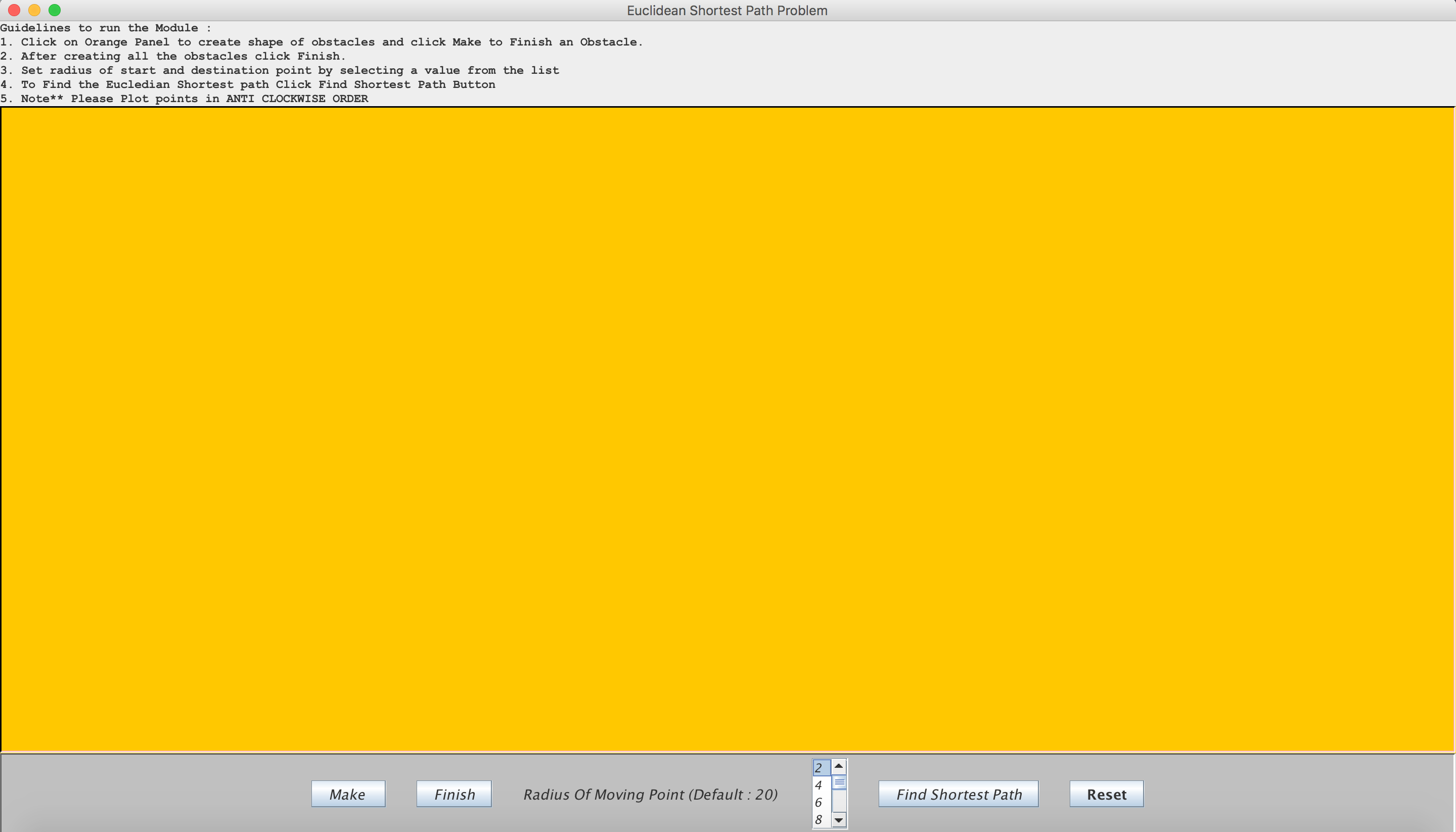
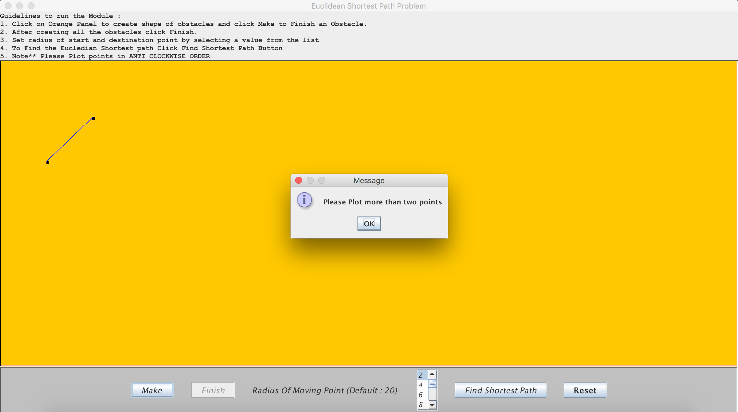
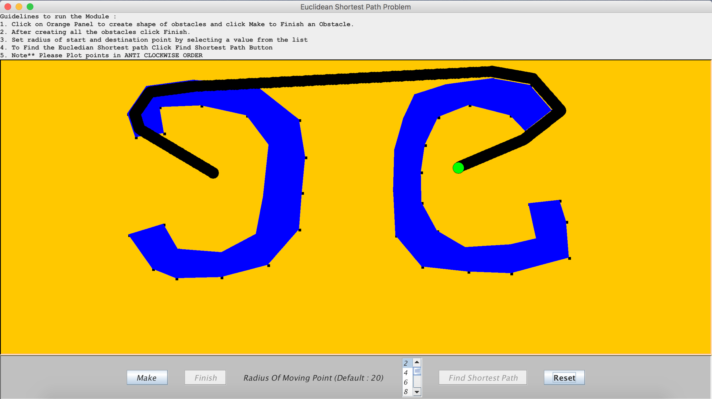
The UI has been implemented using the Swing GUI widget toolkit for Java. The guidelines to be followed are listed right above the canvas. There are a number of buttons provided for efficient functionality. The user can built polygons with mouse clicks on the points where he wants to have a vertex of the polygon and when the last vertex has been plotted, he can close the polygon by clicking on the “MAKE” button which which draw an edge between the first vertex of that polygon and the last vertex just plotted. The user will not be able to proceed if there are two or less than two vertices plotted for a polygon. A polygon needs to have three or more vertices to be closed.

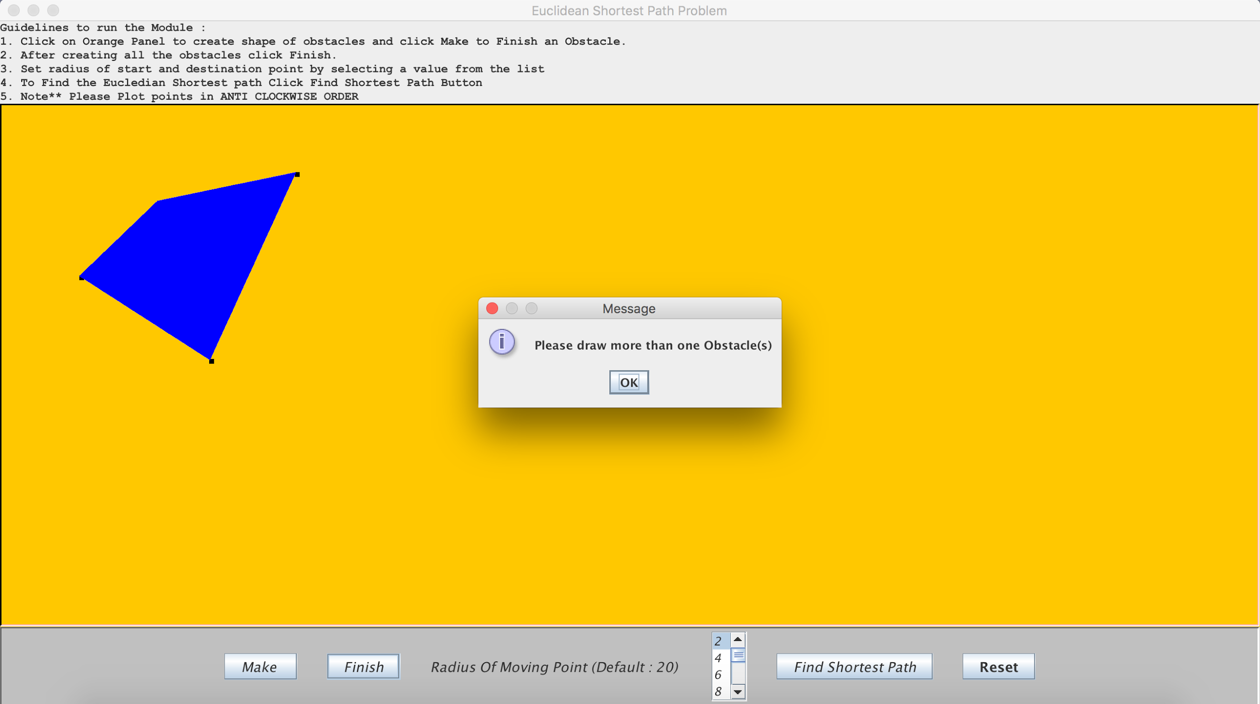
Our algorithm needs the points to be plotted in an anti-clockwise fashion. The validations of the UI are such that it will not let the user proceed until two or more polygons have been drawn. Once the polygons have been drawn, the user can click the “FINISH” button to indicate that he has finished drawing the polygons. It will not let the user pass through this if the last polygon has not been closed.

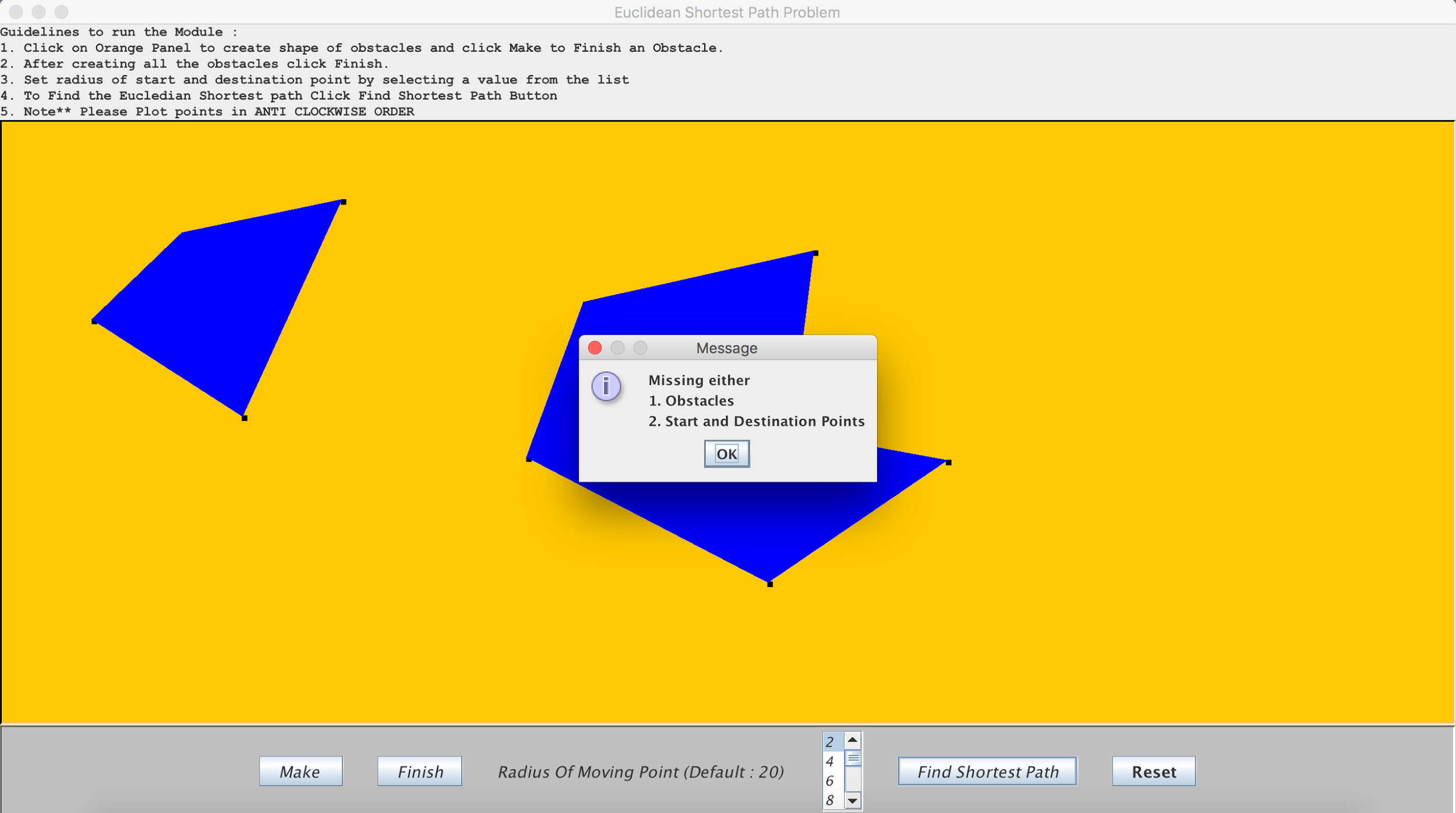
Once the polygons drawn pass through the previous validations, the user can choose the radius of the disk (which is 20 by default) and then select the start and the destination point for the disk object by clicking on the start point and dragging the cursor further without releasing it until the destination point is reached. After that there is a button called “FIND SHORTEST PATH” that starts running the core algorithm. This button will not be valid to be clicked until the start and destination points are fixed else it will give the user a warning in a dialogue box. The click of that button will continue with the steps mentioned further in the algorithm.

The figure below indicates how the UI looks:

2. Compute the convex hull

The concept of convex hull explains the subset of a number of points in a Euclidean plane that envelope the rest of the points in their interior in a convex manner. It is analogous to stretching out a rubber band and snapping it around all the points such that it creates edges with the outermost points. There is a good reason why we planned on computing the convex hull before the core algorithm. In the realistic sense, if a person wants to walk past a building that is concave in shape or around it taking the shortest path, he will always have to walk along the convex hull of the building. If he walks along the concave edges of the building, the total path cost will increase.

There are a number of algorithms to find the convex hull of a number of points in the plane. Jarvis March (also called as Gift Wrapping) starts from the bottommost and leftmost point and wraps around the convex hull by repeatedly identifying the point that has the smallest polar angle with respect to the previous segment drawn from the last two points and adds it to the convex hull in O(nh) time complexity, where n is the total number of points and h is the number of vertices on the convex hull. The Divide and Conquer algorithm computes the convex hull of the left half points and the right half points and then merges the two into a single convex hull result by finding the upper and lower tangents in O(n log n) time complexity, where n is the total number of points. Graham Scan starts with the bottommost and leftmost point and forms the hull by repeatedly identifying the points that make a left turn with the previous segment in O(n log n) time complexity, where n is the total number of points. We have implemented Jarvis’ March and Brute Force Slow algorithm both, but haven’t used either in our application.

3. Inflate the polygons

Movement of a one dimensional point through a bunch of two dimensional obstacles becomes just a problem of visibility. It can be done without any form of collision detection whatsoever. To take advantage of this, we convert this problem to a general visibility problem of a one dimensional point. The way we do this is by reducing the start and the destination circles (the moving circular object) to just their center points, and instead inflating, thickening, or expanding the obstacles outward from their center of gravity with a size or distance equal to the radius of the moving circular object. This essentially remains the same problem but it makes it easy to solve it using just the visibility graph.

We get an inflated polygon by moving the lines representing the polygon edges above or below depending on the direction of the edge by a constant factor. If the edge was made from left vertex to the right vertex then it means that the edge is a lower edge considering that the user is inputting the vertices of an obstacle in counter-clockwise direction. So, in this case we shift the edge below. If the edge is going from a right vertex to a left vertex then it means that that edge is an upper edge and it gets moved above by a constant factor.

Once we know in which direction we are shifting an edge, we have to figure out by how much factor we to shift that edge. We have to move the edge above or below by translating the line along the normal it by a distance equal to the radius of the moving object. This is becomes complicated if we try to compute normals of each and every edge, look for a point that is at a distance of radius along the normal, and then draw a line from that point that is parallel to that edge. We can easily do this by adding or subtracting a value to the y-intercept of the line equation. The value can be found out using some trigonometry.

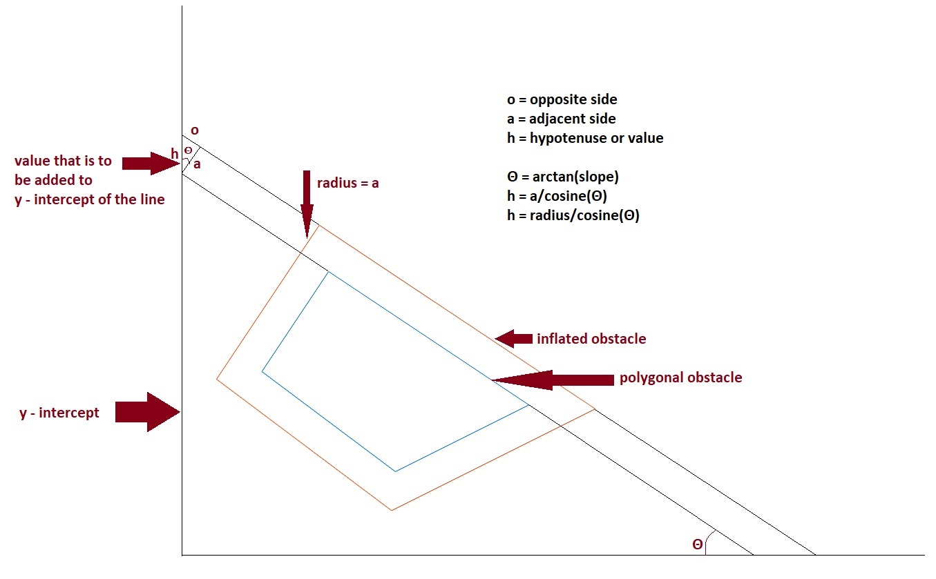
First, we get the angle that the edge/line makes with the x-axis. This will also be the angle that the normal of the line makes with the y-axis.
Θ = tan-1( slope of the line )

Second, we find out the value to be added to the y-intercept. We do that using the formula below.
Value = radius/cos(Θ)

Third, based on whether the edge direction is towards the left or right, we add, or subtract the value from the original y-intercept value.

New y-intercept = old y-intercept + value 		if, x1 < x2
New y-intercept = old y-intercept - value 		if, x2 < x1

This will add or subtract to the old y-intercept and will eventually shift the edge/line above or below with a factor of “value” along the y-axis, or with a factor of “radius” along the normal of the edge/line.

And fourth, we get the intersection points of the new shifted edges that are adjacent to each other. When we are done with finding intersection points of all the adjacent edges, we have our vertices of the inflated polygons ready. And, we do this for all obstacles in our canvas.

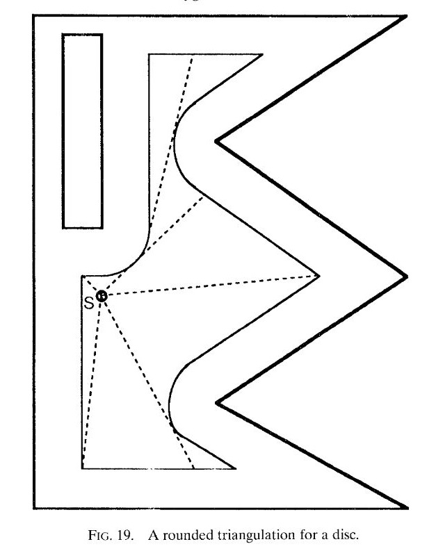
What we call “inflation”, James A. Storer, and John H. Reif call it “padding” in [1]. They have a better approach than ours, considering that they are not doing the approximation of inflation or padding of the corners of the obstacles. When we pad or inflate the obstacles, the edges remain edges, but the corners don’t remain corners, the turn into arcs as shown in Fig 19 of [1].

4. Build the visibility graph

After the inflation has been performed on the polygons and we have its convex hull, we have the final vertices of the polygons. The next step towards finding the shortest path is building a visibility graph since it contains a solution to the shortest path problem. A visibility graph is, as the name suggests, based on the visibility of vertices. The visibility graph contains the vertices of the polygons as the nodes and the edges of the polygons as the edges in the graph. The visibility graph of a polygon, especially concave, would connect vertices of the polygon that can directly connect each other without crossing any other edge of the polygon.

However, the visibility graph of a set of obstacles is a bit different. The graph mostly connects a vertex to the vertices that do not belong to the same polygon. The vertex is connected to a vertex from another polygon if the segment drawn between them does not intersect any other edges of any of the polygons in the plane. In the actual concept of visibility graph of a set of obstacles, no edge is draw between vertices of the same polygon. But in our implementation, vertices belonging to the same polygon are connected only if they are adjacent to each other because movement of the object along the polygon edges is also possible.

There are a couple of approaches to build the visibility graph. An O(n log n) time algorithm uses the binary search tree data structure to build the graph. Another O(n2) algorithm works on the concept of arrangements of lines which refers to the partition of planes that is formed by a collection of lines. An output-sensitive algorithm also exists that runs in O(n log n + E) time, where E is the number of edges in the graph. We have, however, used the naive approach which runs in O(n3) time. For the entire set of vertices it draws a segment to every other vertex that does not belong to the same polygon as itself. Those arrangements would be O(n2). Now, for each arrangement formed, it will check if that segment intersects with any other edge in the entire plane. If it does not intersect with any other edge, then the vertices connected by that segment could be connected in the visibility graph. We also connect adjacent vertices belonging to the same polygon in the graph. In the end, the crucial step is to connect the start and destination points to the vertices of the polygons that it is visible to.

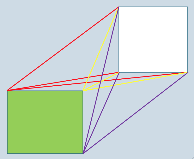
The figure below shows the vertices that the vertices of the green polygon are connected to in the visibility graph. The adjacency list of every vertex is shown by a different color for the ease of visuals. We have only shown the connections between two polygons though, not inter polygonal connectivity. We haven’t shown the vertices being connected to the adjacent vertices of the same polygon because the colors would be overlapped.

5. Implement a shortest path finding algorithm in a graph

We now have the visibility graph built that connects the vertices that the object can traverse through from a vertex. The graph is in the form of an adjacency list rather than an adjacency matrix which allows the traversals to happen in a lesser time complexity while computing the shortest path. Any shortest path algorithm starts its traversal from the start point and checks the vertices it is connected to, building its path by repeating this step in a specific manner based on the algorithm being used, until it reaches a vertex that contains the destination vertex in the list of vertices it is connected to.

The Bellman Ford algorithm finds the shortest path from a source vertex to all other vertices in O(VE) time complexity, where V is the number of nodes in the graph and E is the number of edges. In every iteration it keeps track of the current shortest path for each vertex and considers if the currently formed edge could improve the current shortest path of the vertex at that endpoint. After k iterations, the first k steps of any shortest path are correct and will never change from that point. The Floyd Warshall algorithm finds the shortest path between all the pairs of nodes in the graph in O(V3) time complexity, where V is the number of nodes in the graph. It builds a 3-dimensional dynamic programming array that keeps track of the shortest path between any two vertices, using only some subset of the entire collection of vertices as intermediate steps along the path. We have used Dijkstra’s algorithm that runs in O(V2) time, where V is the number of nodes in the graph. The time complexity can be made better like O(E log V) if a heap data structure is used, but our implementation stays O(V2) since we have used adjacency list.

6. Show visual output

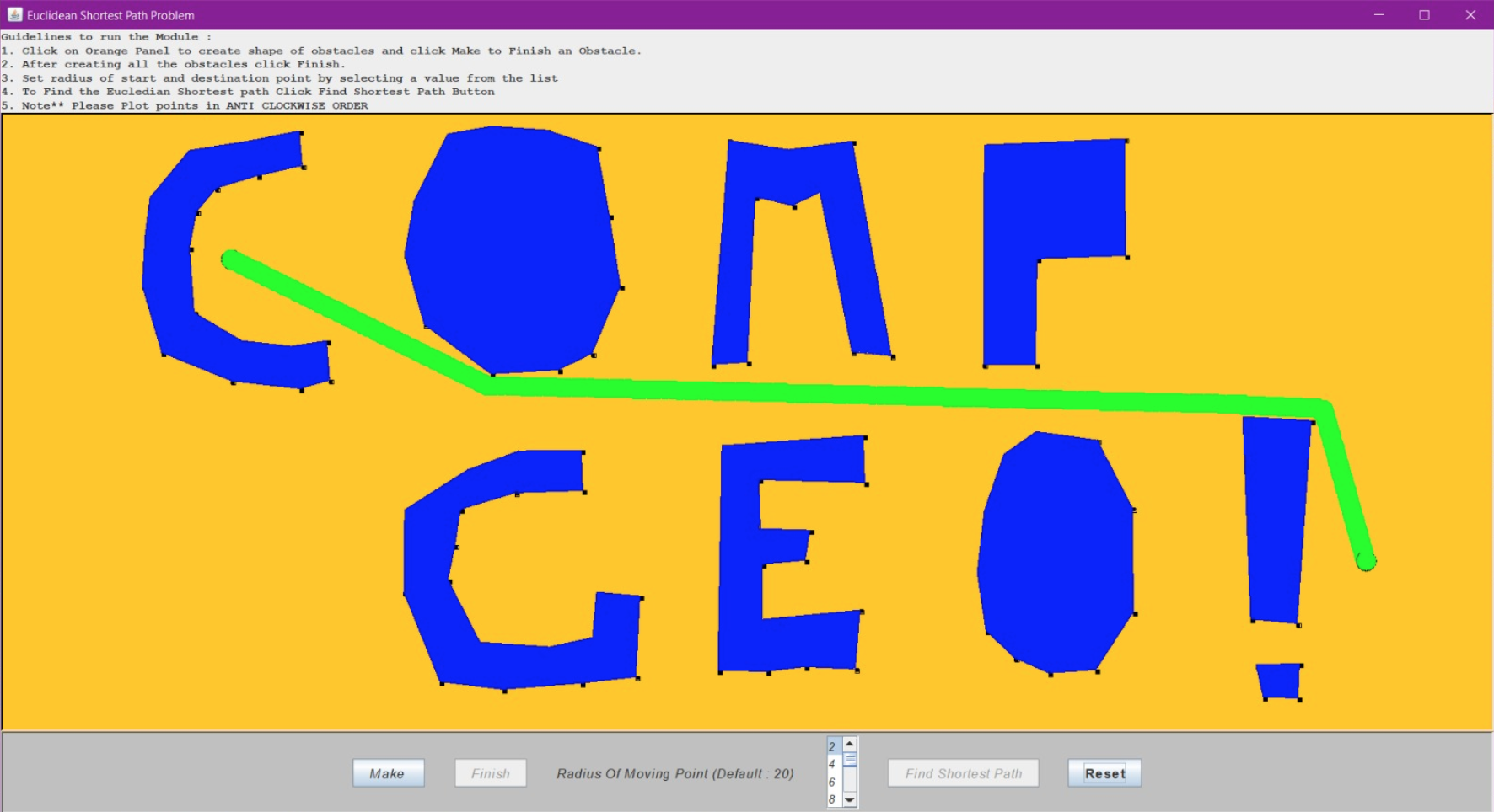
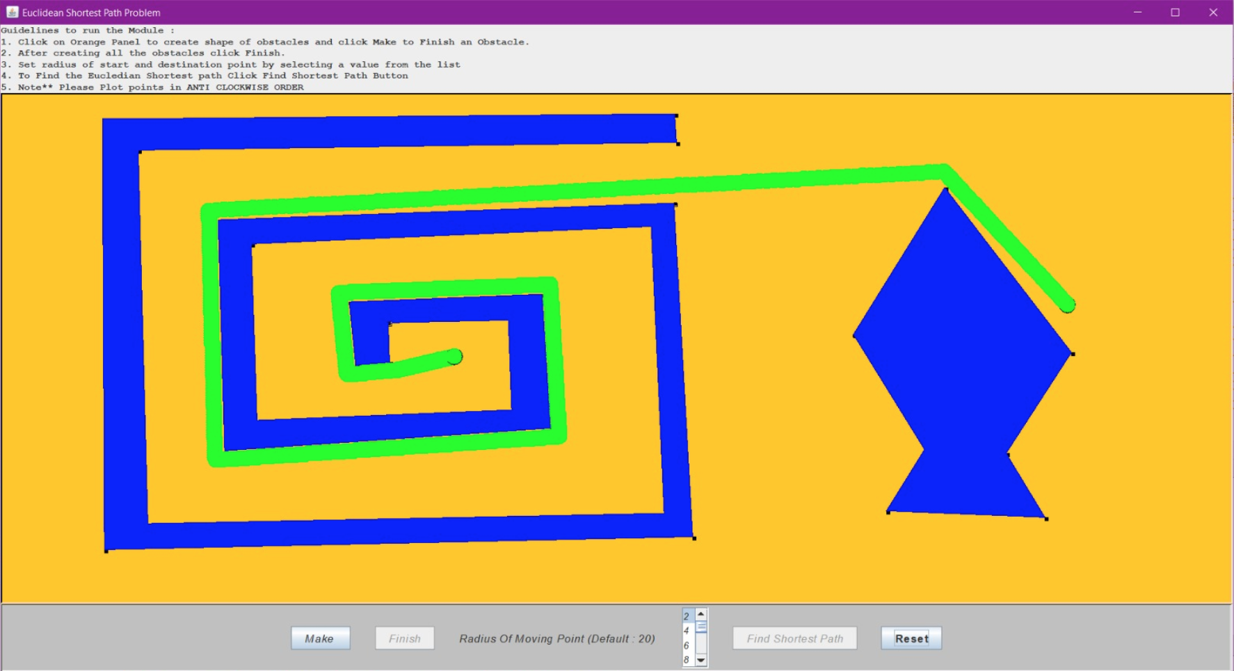
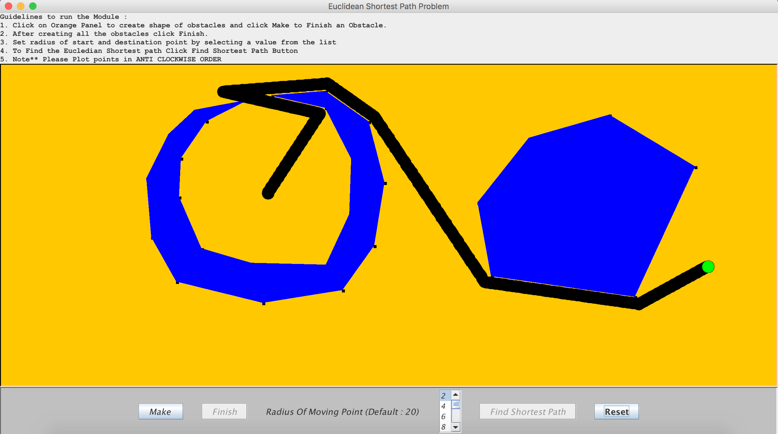
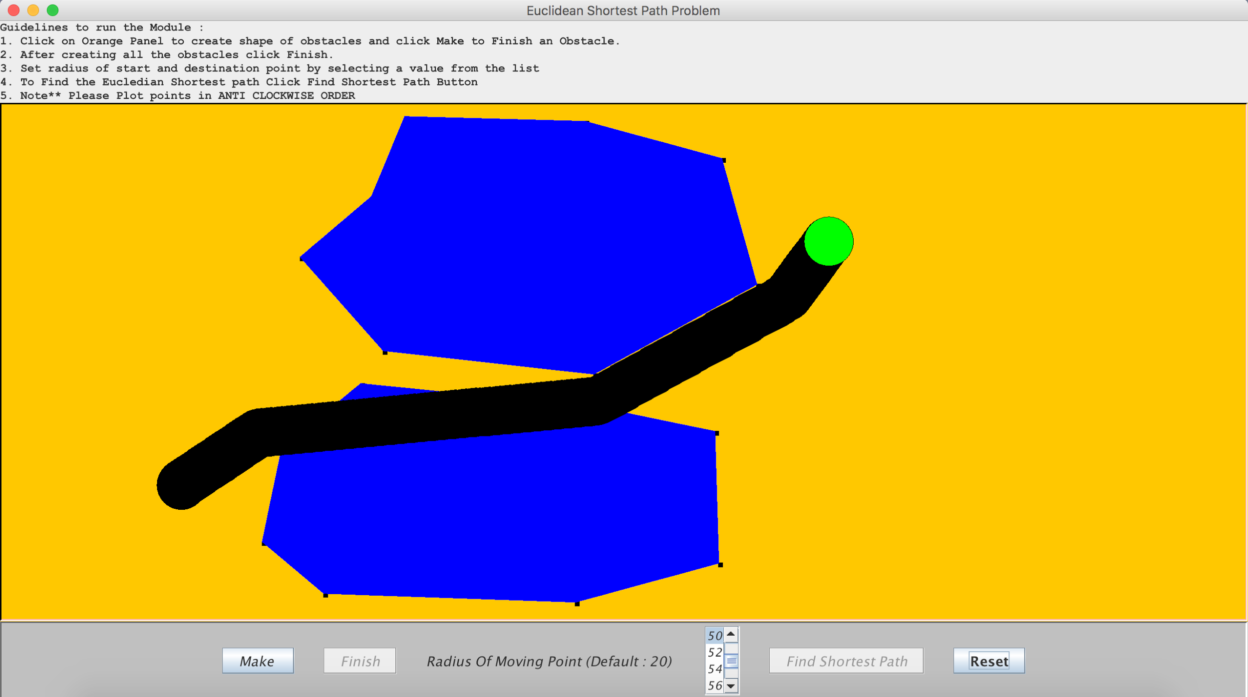
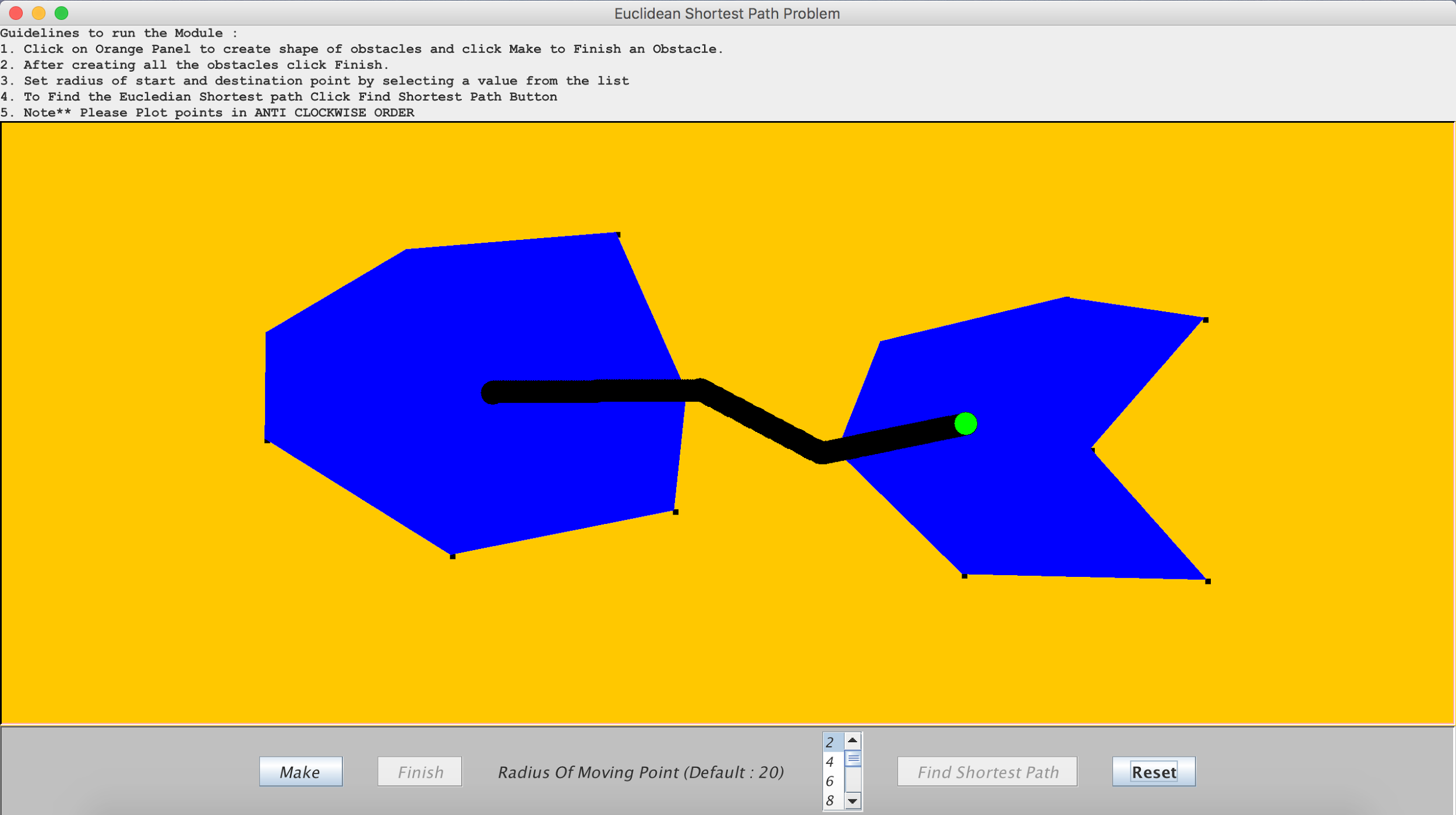
After running the shortest path algorithm on the visibility graph we get a list of output vertices that are a part of the shortest path from the source to the destination point through the obstacles. The path between these output points are animated by interpolating with a fixed fraction between every two adjacent points in the list using the Java Swing toolkit. If the user wants to start off again with new input polygons, he/she can click the “RESET” button to do so.

The figures below show some interesting outputs that we froze:

Validations of the User Interface:

A user interface without validations is not easy to use because the user would not have a guide even when he operates some functions in the wrong way. In that case, the inputs could also be read wrong and would fail some module of the algorithm.

The following validations have been made on our User Interface to make sure that the user is on the right track while creating the inputs:

1. Validation 1: User cannot create an obstacle of two points. The minimum number of points required to create the obstacle is atleast three.

2. Validation 2: The map should contain atleast two obstacles before the user clicks the “FINISH” button.

3. Validation 3: User cannot find the shortest path until all the obstacles are closed and the start and destination points have been plotted.

Limitations:

Although we have tried to develop an algorithm that would work in most input scenarios, there are certain cases where our algorithm fails. Some reasons to this include concave polygons not being handled when visibility graph is built, inflation of polygons with vertex points at edges instead of curved arcs, etc.

1. Scenario 1: The obstacles contain sharp edges that are in close vicinity of each other.

2. Scenario 2: The radius of the moving circular disk does not fit in the path that leads to the destination point.

3. Scenario 3: The start or destination point or both the points lie within an obstacle.

4. Scenario 4: The obstacle vertices are plotted in a clockwise fashion.

Future Work:

Our algorithm can be further be improvised on in a number of aspects. For our stretched goals with respect to this implementation, we can firstly fix our limitation scenarios. For Scenario 1, we can revise the way we inflate our polygons. Instead of having it inflated into new vertices, we can inflate the portions close to the edges as arcs to maintain the closest approximation of the radius of the circular moving object all around the polygon. The math involved would be more complicated and we would end up having multiple vertices along the curves of the vertices that would in turn increase the computation time. For Scenario 2, we can have perpendiculars drawn from every endpoint to every other edge where the perpendicular does not intersect any intermediate edges. This is the naive approach to it, unless there exists some math that could easily solve this. For Scenario 3, we can have nothing but a validation in the User Interface that checks if the start or destination point lies inside a polygon that has been made by the user, and give a warning along with another chance of selecting the start and destination points until they seem fit. For Scenario 4, we can check the orientation in which the vertices of every polygon are plotted. If the vertices for any polygon have been plotted in the clockwise manner, modify it to be anti-clockwise before using it as an input to the algorithm. The key here is to detect the orientation of the vertices.

Another major way in which we could extend this algorithm is by allowing the moving object to be a two dimensional rectangle. The rectangle would have to check whether it fits within the space between two vertex ends or between the edges (parallel or nonparallel) of two different polygons. This would involve a huge number of computations since the object would have to be rotated with small incrementations repeated and checked for intersections with the edges of the polygons multiple times. This is not a feasible method to follow since we would not know its final computation time.

Source Code:

Find files of our Shortest Path tool here!

References:

1. [1] “Shortest Path in the Plane with Polygonal Obstacles”, James A. Storer, John H. Reif, Journal of the ACM (JACM) 5 September, 1994, pp. 982 - 1012.
2. [2] “Computing Shortest Paths among Curved Obstacles in the Plane”, Danny Z. Chen, Haitao Wang, ACM Transactions on Algorithms, Vol. 11(4), Article No. 26, 2015.
3. [3] “Deriving an Obstacle-Avoiding Shortest Path in Continuous Space: A Spatial Analytic Approach”, Insu Hong, Arizona State University, May 2015.
4. [4] “Complexity of the generalized mover’s problem”, John H. Reif, 1979.